Hints for Performance Tuning#
This chapter provides hints on how to get to achieve best performance with PETSc, particularly on distributed-memory machines with multiple CPU sockets per node. We focus on machine-related performance optimization here; algorithmic aspects like preconditioner selection are not the focus of this section.
Maximizing Memory Bandwidth#
Most operations in PETSc deal with large datasets (typically vectors and sparse matrices) and perform relatively few arithmetic operations for each byte loaded or stored from global memory. Therefore, the arithmetic intensity expressed as the ratio of floating point operations to the number of bytes loaded and stored is usually well below unity for typical PETSc operations. On the other hand, modern CPUs are able to execute on the order of 10 floating point operations for each byte loaded or stored. As a consequence, almost all PETSc operations are limited by the rate at which data can be loaded or stored (memory bandwidth limited) rather than by the rate of floating point operations.
This section discusses ways to maximize the memory bandwidth achieved by applications based on PETSc. Where appropriate, we include benchmark results in order to provide quantitative results on typical performance gains one can achieve through parallelization, both on a single compute node and across nodes. In particular, we start with the answer to the common question of why performance generally does not increase 20-fold with a 20-core CPU.
Memory Bandwidth vs. Processes#
Consider the addition of two large vectors, with the result written to a third vector. Because there are no dependencies across the different entries of each vector, the operation is embarrasingly parallel.
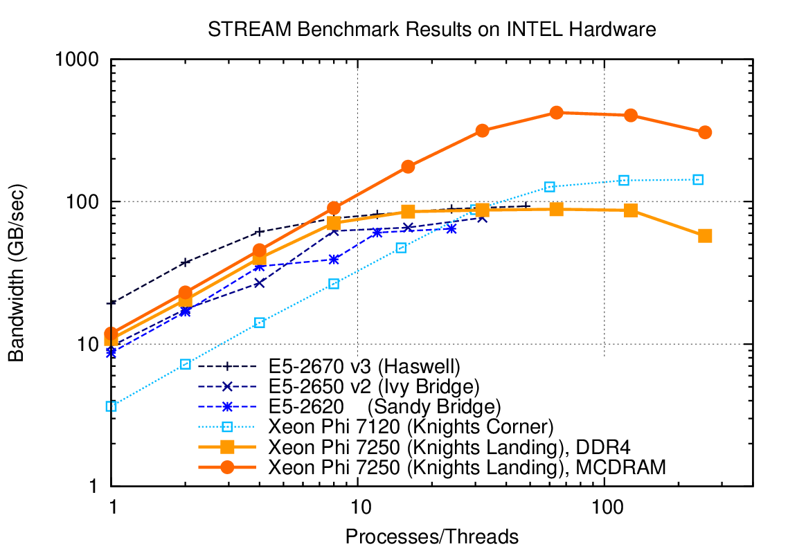
Fig. 14 Memory bandwidth obtained on Intel hardware (dual socket except KNL) over the number of processes used. One can get close to peak memory bandwidth with only a few processes.#
As Fig. 14 shows, the performance gains due to parallelization on different multi- and many-core CPUs quickly saturates. The reason is that only a fraction of the total number of CPU cores is required to saturate the memory channels. For example, a dual-socket system equipped with Haswell 12-core Xeon CPUs achieves more than 80 percent of achievable peak memory bandwidth with only four processes per socket (8 total), cf. Fig. 14. Consequently, running with more than 8 MPI ranks on such a system will not increase performance substantially. For the same reason, PETSc-based applications usually do not benefit from hyper-threading.
PETSc provides a simple way to measure memory bandwidth for different
numbers of processes via the target make streams executed from
$PETSC_DIR. The output provides an overview of the possible speedup
one can obtain on the given machine (not necessarily a shared memory
system). For example, the following is the most relevant output obtained
on a dual-socket system equipped with two six-core-CPUs with
hyperthreading:
np  speedup
1 1.0
2 1.58
3 2.19
4 2.42
5 2.63
6 2.69
...
21 3.82
22 3.49
23 3.79
24 3.71
Estimation of possible speedup of MPI programs based on Streams benchmark.
It appears you have 1 node(s)
On this machine, one should expect a speed-up of typical memory bandwidth-bound PETSc applications of at most 4x when running multiple MPI ranks on the node. Most of the gains are already obtained when running with only 4-6 ranks. Because a smaller number of MPI ranks usually implies better preconditioners and better performance for smaller problems, the best performance for PETSc applications may be obtained with fewer ranks than there are physical CPU cores available.
Following the results from the above run of make streams, we
recommend to use additional nodes instead of placing additional MPI
ranks on the nodes. In particular, weak scaling (i.e. constant load per
process, increasing the number of processes) and strong scaling
(i.e. constant total work, increasing the number of processes) studies
should keep the number of processes per node constant.
Non-Uniform Memory Access (NUMA) and Process Placement#
CPUs in nodes with more than one CPU socket are internally connected via a high-speed fabric, cf. Fig. 15, to enable data exchange as well as cache coherency. Because main memory on modern systems is connected via the integrated memory controllers on each CPU, memory is accessed in a non-uniform way: A process running on one socket has direct access to the memory channels of the respective CPU, whereas requests for memory attached to a different CPU socket need to go through the high-speed fabric. Consequently, best aggregate memory bandwidth on the node is obtained when the memory controllers on each CPU are fully saturated. However, full saturation of memory channels is only possible if the data is distributed across the different memory channels.

Fig. 15 Schematic of a two-socket NUMA system. Processes should be spread across both CPUs to obtain full bandwidth.#
Data in memory on modern machines is allocated by the operating system
based on a first-touch policy. That is, memory is not allocated at the
point of issuing malloc(), but at the point when the respective
memory segment is actually touched (read or write). Upon first-touch,
memory is allocated on the memory channel associated with the respective
CPU the process is running on. Only if all memory on the respective CPU
is already in use (either allocated or as IO cache), memory available
through other sockets is considered.
Maximum memory bandwidth can be achieved by ensuring that processes are
spread over all sockets in the respective node. For example, the
recommended placement of a 8-way parallel run on a four-socket machine
is to assign two processes to each CPU socket. To do so, one needs to
know the enumeration of cores and pass the requested information to
mpirun. Consider the hardware topology information returned by
lstopo (part of the hwloc package) for the following two-socket
machine, in which each CPU consists of six cores and supports
hyperthreading:
Machine (126GB total)
  NUMANode L#0 (P#0 63GB)
    Package L#0 + L3 L#0 (15MB)
      L2 L#0 (256KB) + L1d L#0 (32KB) + L1i L#0 (32KB) + Core L#0
        PU L#0 (P#0)
        PU L#1 (P#12)
      L2 L#1 (256KB) + L1d L#1 (32KB) + L1i L#1 (32KB) + Core L#1
        PU L#2 (P#1)
        PU L#3 (P#13)
      L2 L#2 (256KB) + L1d L#2 (32KB) + L1i L#2 (32KB) + Core L#2
        PU L#4 (P#2)
        PU L#5 (P#14)
      L2 L#3 (256KB) + L1d L#3 (32KB) + L1i L#3 (32KB) + Core L#3
        PU L#6 (P#3)
        PU L#7 (P#15)
      L2 L#4 (256KB) + L1d L#4 (32KB) + L1i L#4 (32KB) + Core L#4
        PU L#8 (P#4)
        PU L#9 (P#16)
      L2 L#5 (256KB) + L1d L#5 (32KB) + L1i L#5 (32KB) + Core L#5
        PU L#10 (P#5)
        PU L#11 (P#17)
  NUMANode L#1 (P#1 63GB)
    Package L#1 + L3 L#1 (15MB)
      L2 L#6 (256KB) + L1d L#6 (32KB) + L1i L#6 (32KB) + Core L#6
        PU L#12 (P#6)
        PU L#13 (P#18)
      L2 L#7 (256KB) + L1d L#7 (32KB) + L1i L#7 (32KB) + Core L#7
        PU L#14 (P#7)
        PU L#15 (P#19)
      L2 L#8 (256KB) + L1d L#8 (32KB) + L1i L#8 (32KB) + Core L#8
        PU L#16 (P#8)
        PU L#17 (P#20)
      L2 L#9 (256KB) + L1d L#9 (32KB) + L1i L#9 (32KB) + Core L#9
        PU L#18 (P#9)
        PU L#19 (P#21)
      L2 L#10 (256KB) + L1d L#10 (32KB) + L1i L#10 (32KB) + Core L#10
        PU L#20 (P#10)
        PU L#21 (P#22)
      L2 L#11 (256KB) + L1d L#11 (32KB) + L1i L#11 (32KB) + Core L#11
        PU L#22 (P#11)
        PU L#23 (P#23)
The relevant physical processor IDs are shown in parentheses prefixed by
P#. Here, IDs 0 and 12 share the same physical core and have a
common L2 cache. IDs 0, 12, 1, 13, 2, 14, 3, 15, 4, 16, 5, 17 share the
same socket and have a common L3 cache.
A good placement for a run with six processes is to locate three
processes on the first socket and three processes on the second socket.
Unfortunately, mechanisms for process placement vary across MPI
implementations, so make sure to consult the manual of your MPI
implementation. The following discussion is based on how processor
placement is done with MPICH and Open MPI, where one needs to pass
--bind-to core --map-by socket to mpirun:
$ mpirun -n 6 --bind-to core --map-by socket ./stream
process 0 binding: 100000000000100000000000
process 1 binding: 000000100000000000100000
process 2 binding: 010000000000010000000000
process 3 binding: 000000010000000000010000
process 4 binding: 001000000000001000000000
process 5 binding: 000000001000000000001000
Triad:        45403.1949   Rate (MB/s)
In this configuration, process 0 is bound to the first physical core on the first socket (with IDs 0 and 12), process 1 is bound to the first core on the second socket (IDs 6 and 18), and similarly for the remaining processes. The achieved bandwidth of 45 GB/sec is close to the practical peak of about 50 GB/sec available on the machine. If, however, all MPI processes are located on the same socket, memory bandwidth drops significantly:
$ mpirun -n 6 --bind-to core --map-by core ./stream
process 0 binding: 100000000000100000000000
process 1 binding: 010000000000010000000000
process 2 binding: 001000000000001000000000
process 3 binding: 000100000000000100000000
process 4 binding: 000010000000000010000000
process 5 binding: 000001000000000001000000
Triad:        25510.7507   Rate (MB/s)
All processes are now mapped to cores on the same socket. As a result, only the first memory channel is fully saturated at 25.5 GB/sec.
mpirun uses good defaults. To
demonstrate, compare the full output of make streams from
Memory Bandwidth vs. Processes on the left with
the results on the right obtained by passing
--bind-to core --map-by socket:$ make streams
np speedup
1 1.0
2 1.58
3 2.19
4 2.42
5 2.63
6 2.69
7 2.31
8 2.42
9 2.37
10 2.65
11 2.3
12 2.53
13 2.43
14 2.63
15 2.74
16 2.7
17 3.28
18 3.66
19 3.95
20 3.07
21 3.82
22 3.49
23 3.79
24 3.71
$ make streams MPI_BINDING="--bind-to core --map-by socket"
np  speedup
1 1.0
2 1.59
3 2.66
4 3.5
5 3.56
6 4.23
7 3.95
8 4.39
9 4.09
10 4.46
11 4.15
12 4.42
13 3.71
14 3.83
15 4.08
16 4.22
17 4.18
18 4.31
19 4.22
20 4.28
21 4.25
22 4.23
23 4.28
24 4.22
make streams with proper processor placement shown on the right
resulted in slightly higher overall parallel speedup (identical
baselines), in smaller performance fluctuations, and more than 90
percent of peak bandwidth with only six processes.Machines with job submission systems such as SLURM usually provide similar mechanisms for processor placements through options specified in job submission scripts. Please consult the respective manuals.
Additional Process Placement Considerations and Details#
For a typical, memory bandwidth-limited PETSc application, the primary consideration in placing MPI processes is ensuring that processes are evenly distributed among sockets, and hence using all available memory channels. Increasingly complex processor designs and cache hierarchies, however, mean that performance may also be sensitive to how processes are bound to the resources within each socket. Performance on the two processor machine in the preceding example may be relatively insensitive to such placement decisions, because one L3 cache is shared by all cores within a NUMA domain, and each core has its own L2 and L1 caches. However, processors that are less “flat”, with more complex hierarchies, may be more sensitive. In many AMD Opterons or the second-generation “Knights Landing” Intel Xeon Phi, for instance, L2 caches are shared between two cores. On these processors, placing consecutive MPI ranks on cores that share the same L2 cache may benefit performance if the two ranks communicate frequently with each other, because the latency between cores sharing an L2 cache may be roughly half that of two cores not sharing one. There may be benefit, however, in placing consecutive ranks on cores that do not share an L2 cache, because (if there are fewer MPI ranks than cores) this increases the total L2 cache capacity and bandwidth available to the application. There is a trade-off to be considered between placing processes close together (in terms of shared resources) to optimize for efficient communication and synchronization vs. farther apart to maximize available resources (memory channels, caches, I/O channels, etc.), and the best strategy will depend on the application and the software and hardware stack.
Different process placement strategies can affect performance at least
as much as some commonly explored settings, such as compiler
optimization levels. Unfortunately, exploration of this space is
complicated by two factors: First, processor and core numberings may be
completely arbitrary, changing with BIOS version, etc., and second—as
already noted—there is no standard mechanism used by MPI implementations
(or job schedulers) to specify process affinity. To overcome the first
issue, we recommend using the lstopo utility of the Portable
Hardware Locality (hwloc) software package (which can be installed
by configuring PETSc with –download-hwloc) to understand the
processor topology of your machine. We cannot fully address the second
issue—consult the documenation for your MPI implementation and/or job
scheduler—but we offer some general observations on understanding
placement options:
An MPI implementation may support a notion of domains in which a process may be pinned. A domain may simply correspond to a single core; however, the MPI implementation may allow a deal of flexibility in specifying domains that encompass multiple cores, span sockets, etc. Some implementations, such as Intel MPI, provide means to specify whether domains should be “compact”—composed of cores sharing resources such as caches—or “scatter”-ed, with little resource sharing (possibly even spanning sockets).
Separate from the specification of domains, MPI implementations often support different orderings in which MPI ranks should be bound to these domains. Intel MPI, for instance, supports “compact” ordering to place consecutive ranks close in terms of shared resources, “scatter” to place them far apart, and “bunch” to map proportionally to sockets while placing ranks as close together as possible within the sockets.
An MPI implemenation that supports process pinning should offer some way to view the rank assignments. Use this output in conjunction with the topology obtained via
lstopoor a similar tool to determine if the placements correspond to something you believe is reasonable for your application. Do not assume that the MPI implementation is doing something sensible by default!
Performance Pitfalls and Advice#
This section looks into a potpourri of performance pitfalls encountered by users in the past. Many of these pitfalls require a deeper understanding of the system and experience to detect. The purpose of this section is to summarize and share our experience so that these pitfalls can be avoided in the future.
Debug vs. Optimized Builds#
PETSc’s configure defaults to building PETSc with debug mode
enabled. Any code development should be done in this mode, because it
provides handy debugging facilities such as accurate stack traces,
memory leak checks, and memory corruption checks. Note that PETSc has no
reliable way of knowing whether a particular run is a production or
debug run. In the case that a user requests profiling information via
-log_view, a debug build of PETSc issues the following warning:
##########################################################
#                                                        #
#                          WARNING!!!                    #
#                                                        #
#   This code was compiled with a debugging option,      #
#   To get timing results run configure                  #
#   using --with-debugging=no, the performance will      #
#   be generally two or three times faster.              #
#                                                        #
##########################################################
Conversely, one way of checking whether a particular build of PETSc has
debugging enabled is to inspect the output of -log_view.
Debug mode will generally be most useful for code development if
appropriate compiler options are set to faciliate debugging. The
compiler should be instructed to generate binaries with debug symbols
(command line option -g for most compilers), and the optimization
level chosen should either completely disable optimizations (-O0 for
most compilers) or enable only optimizations that do not interfere with
debugging (GCC, for instance, supports a -Og optimization level that
does this).
Only once the new code is thoroughly tested and ready for production,
one should disable debugging facilities by passing
--with-debugging=no to
configure. One should also ensure that an appropriate compiler
optimization level is set. Note that some compilers (e.g., Intel)
default to fairly comprehensive optimization levels, while others (e.g.,
GCC) default to no optimization at all. The best optimization flags will
depend on your code, the compiler, and the target architecture, but we
offer a few guidelines for finding those that will offer the best
performance:
Most compilers have a number of optimization levels (with level n usually specified via
-On) that provide a quick way to enable sets of several optimization flags. We suggest trying the higher optimization levels (the highest level is not guaranteed to produce the fastest executable, so some experimentation may be merited). With most recent processors now supporting some form of SIMD or vector instructions, it is important to choose a level that enables the compiler’s auto-vectorizer; many compilers do not enable auto-vectorization at lower optimization levels (e.g., GCC does not enable it below-O3and the Intel compiler does not enable it below-O2).For processors supporting newer vector instruction sets, such as Intel AVX2 and AVX-512, it is also important to direct the compiler to generate code that targets these processors (e.g.,
-march=native); otherwise, the executables built will not utilize the newer instructions sets and will not take advantage of the vector processing units.Beyond choosing the optimization levels, some value-unsafe optimizations (such as using reciprocals of values instead of dividing by those values, or allowing re-association of operands in a series of calculations) for floating point calculations may yield significant performance gains. Compilers often provide flags (e.g.,
-ffast-mathin GCC) to enable a set of these optimizations, and they may be turned on when using options for very aggressive optimization (-fastor-Ofastin many compilers). These are worth exploring to maximize performance, but, if employed, it important to verify that these do not cause erroneous results with your code, since calculations may violate the IEEE standard for floating-point arithmetic.
Profiling#
Users should not spend time optimizing a code until after having determined where it spends the bulk of its time on realistically sized problems. As discussed in detail in Profiling, the PETSc routines automatically log performance data if certain runtime options are specified.
To obtain a summary of where and how much time is spent in different sections of the code, use one of the following options:
Run the code with the option
-log_viewto print a performance summary for various phases of the code.Run the code with the option
-log_mpe[logfilename], which creates a logfile of events suitable for viewing with Jumpshot (part of MPICH).
Then, focus on the sections where most of the time is spent. If you
provided your own callback routines, e.g. for residual evaluations,
search the profiling output for routines such as SNESFunctionEval or
SNESJacobianEval. If their relative time is significant (say, more
than 30 percent), consider optimizing these routines first. Generic
instructions on how to optimize your callback functions are difficult;
you may start by reading performance optimization guides for your
system’s hardware.
Aggregation#
Performing operations on chunks of data rather than a single element at a time can significantly enhance performance because of cache reuse or lower data motion. Typical examples are:
Insert several (many) elements of a matrix or vector at once, rather than looping and inserting a single value at a time. In order to access elements in of vector repeatedly, employ
VecGetArray()to allow direct manipulation of the vector elements.When possible, use
VecMDot()rather than a series of calls toVecDot().If you require a sequence of matrix-vector products with the same matrix, consider packing your vectors into a single matrix and use matrix-matrix multiplications.
Users should employ a reasonable number of
PetscMalloc()calls in their codes. Hundreds or thousands of memory allocations may be appropriate; however, if tens of thousands are being used, then reducing the number ofPetscMalloc()calls may be warranted. For example, reusing space or allocating large chunks and dividing it into pieces can produce a significant savings in allocation overhead. Data Structure Reuse gives details.
Aggressive aggregation of data may result in inflexible datastructures and code that is hard to maintain. We advise users to keep these competing goals in mind and not blindly optimize for performance only.
Memory Allocation for Sparse Matrix Factorization#
When symbolically factoring an AIJ matrix, PETSc has to guess how much
fill there will be. Careful use of the fill parameter in the
MatFactorInfo structure when calling MatLUFactorSymbolic() or
MatILUFactorSymbolic() can reduce greatly the number of mallocs and
copies required, and thus greatly improve the performance of the
factorization. One way to determine a good value for the fill parameter
is to run a program with the option -info. The symbolic
factorization phase will then print information such as
Info:MatILUFactorSymbolic_SeqAIJ:Reallocs 12 Fill ratio:given 1 needed 2.16423
This indicates that the user should have used a fill estimate factor of about 2.17 (instead of 1) to prevent the 12 required mallocs and copies. The command line option
-pc_factor_fill 2.17
will cause PETSc to preallocate the correct amount of space for the factorization.
Detecting Memory Allocation Problems and Memory Usage#
PETSc provides tools to aid in understanding PETSc memory usage and detecting problems with
memory allocation, including leaks and use of uninitialized space. Internally, PETSc uses
the routines PetscMalloc() and PetscFree() for memory allocation; instead of directly calling malloc() and free().
This allows PETSc to track its memory usage and perform error checking. Users are urged to use these routines as well when
appropriate.
The option
-malloc_debugturns on PETSc’s extensive runtime error checking of memory for corruption. This checking can be expensive, so should not be used for production runs. The option-malloc_testis equivalent to-malloc_debugbut only works when PETSc is configured with--with-debugging(the default configuration). We suggest setting the environmental variablePETSC_OPTIONS=-malloc_testin your shell startup file to automatically enable runtime check memory for developing code but not running optimized code. Using-malloc_debugor-malloc_testfor large runs can slow them significantly, thus we recommend turning them off if you code is painfully slow and you don’t need the testing. In addition, you can use-check_pointer_intensity 0for long run debug runs that do not need extensive memory corruption testing. This option is occasionally added to thePETSC_OPTIONSenvironmental variable by some users.The option
-malloc_dumpwill print a list of memory locations that have not been freed at the conclusion of a program. If all memory has been freed no message is printed. Note that the option-malloc_dumpactivates a call toPetscMallocDump()duringPetscFinalize(). The user can also callPetscMallocDump()elsewhere in a program.Another useful option is
-malloc_view, which reports memory usage in all routines at the conclusion of the program. Note that this option activates logging by callingPetscMallocViewSet()inPetscInitialize()and then prints the log by callingPetscMallocView()inPetscFinalize(). The user can also call these routines elsewhere in a program.When finer granularity is desired, the user can call
PetscMallocGetCurrentUsage()andPetscMallocGetMaximumUsage()for memory allocated by PETSc, orPetscMemoryGetCurrentUsage()andPetscMemoryGetMaximumUsage()for the total memory used by the program. Note thatPetscMemorySetGetMaximumUsage()must be called beforePetscMemoryGetMaximumUsage()(typically at the beginning of the program).The option
-memory_viewprovides a high-level view of all memory usage, not just the memory used byPetscMalloc(), at the conclusion of the program.When running with
-log_view, the additional option-log_view_memorycauses the display of additional columns of information about how much memory was allocated and freed during each logged event. This is useful to understand what phases of a computation require the most memory.
One can also use Valgrind to track memory usage and find bugs, see FAQ: Valgrind usage.
Data Structure Reuse#
Data structures should be reused whenever possible. For example, if a code often creates new matrices or vectors, there often may be a way to reuse some of them. Very significant performance improvements can be achieved by reusing matrix data structures with the same nonzero pattern. If a code creates thousands of matrix or vector objects, performance will be degraded. For example, when solving a nonlinear problem or timestepping, reusing the matrices and their nonzero structure for many steps when appropriate can make the code run significantly faster.
A simple technique for saving work vectors, matrices, etc. is employing a user-defined context. In C and C++ such a context is merely a structure in which various objects can be stashed; in Fortran a user context can be an integer array that contains both parameters and pointers to PETSc objects. See SNES Tutorial ex5 and SNES Tutorial ex5f90 for examples of user-defined application contexts in C and Fortran, respectively.
Numerical Experiments#
PETSc users should run a variety of tests. For example, there are a large number of options for the linear and nonlinear equation solvers in PETSc, and different choices can make a very big difference in convergence rates and execution times. PETSc employs defaults that are generally reasonable for a wide range of problems, but clearly these defaults cannot be best for all cases. Users should experiment with many combinations to determine what is best for a given problem and customize the solvers accordingly.
Use the options
-snes_view,-ksp_view, etc. (or the routinesKSPView(),SNESView(), etc.) to view the options that have been used for a particular solver.Run the code with the option
-helpfor a list of the available runtime commands.Use the option
-infoto print details about the solvers’ operation.Use the PETSc monitoring discussed in Profiling to evaluate the performance of various numerical methods.
Tips for Efficient Use of Linear Solvers#
As discussed in KSP: Linear System Solvers, the default linear solvers are
- uniprocess: GMRES(30) with ILU(0) preconditioning
- multiprocess: GMRES(30) with block Jacobi preconditioning, where there is 1 block per process, and each block is solved with ILU(0)
One should experiment to determine alternatives that may be better for
various applications. Recall that one can specify the KSP methods
and preconditioners at runtime via the options:
-ksp_type <ksp_name> -pc_type <pc_name>
One can also specify a variety of runtime customizations for the solvers, as discussed throughout the manual.
In particular, note that the default restart parameter for GMRES is 30,
which may be too small for some large-scale problems. One can alter this
parameter with the option -ksp_gmres_restart <restart> or by calling
KSPGMRESSetRestart(). Krylov Methods gives
information on setting alternative GMRES orthogonalization routines,
which may provide much better parallel performance.
For elliptic problems one often obtains good performance and scalability with multigrid solvers. Consult Algebraic Multigrid (AMG) Preconditioners for available options. Our experience is that GAMG works particularly well for elasticity problems, whereas hypre does well for scalar problems.