
Matrices#
PETSc provides a variety of matrix implementations because no single matrix format is appropriate for all problems. Currently, we support dense storage and compressed sparse row storage (both sequential and parallel versions) for CPU and GPU based matrices, as well as several specialized formats. Additional specialized formats can be easily added.
This chapter describes the basics of using PETSc matrices in general (regardless of the particular format chosen) and discusses tips for efficient use of the several simple uniprocess and parallel matrix types. The use of PETSc matrices involves the following actions: create a particular type of matrix, insert values into it, process the matrix, use the matrix for various computations, and finally destroy the matrix. The application code does not need to know or care about the particular storage formats of the matrices.
Creating matrices#
As with vectors, PETSc has APIs that allow the user to specify the exact details of the matrix
creation process but also DM based creation routines that handle most of the details automatically
for specific families of applications. This is done with
DMCreateMatrix(DM dm,Mat *A)
The type of matrix created can be controlled with either
DMSetMatType(DM dm,MatType <MATAIJ or MATBAIJ or MATAIJCUSPARSE etc>)
or with
DMSetFromOptions(DM dm)
and the options database option -dm_mat_type (aij|baij|aijcusparse|...) Matrices can be created for CPU usage, for GPU usage and for usage on
both the CPUs and GPUs.
The creation of DM objects is discussed in DMDA - Creating vectors for structured grids, DMPLEX - Creating vectors for unstructured grids, DMNETWORK - Creating vectors for networks.
Low-level matrix creation routines#
When using a DM is not practical for a particular application one can create matrices directly
using
This routine generates a sequential matrix when running one process and
a parallel matrix for two or more processes; the particular matrix
format is set by the user via options database commands. The user
specifies either the global matrix dimensions, given by M and N
or the local dimensions, given by m and n while PETSc completely
controls memory allocation. This routine facilitates switching among
various matrix types, for example, to determine the format that is most
efficient for a certain application. By default, MatCreate() employs
the sparse AIJ format, which is discussed in detail in
Sparse Matrices. See the manual pages for further
information about available matrix formats.
Assembling (putting values into) matrices#
To insert or add entries to a matrix on CPUs, one can call a variant of
MatSetValues(), either
MatSetValues(Mat A,PetscInt m,const PetscInt idxm[],PetscInt n,const PetscInt idxn[],const PetscScalar values[],INSERT_VALUES);
or
MatSetValues(Mat A,PetscInt m,const PetscInt idxm[],PetscInt n,const PetscInt idxn[],const PetscScalar values[],ADD_VALUES);
This routine inserts or adds a logically dense subblock of dimension
m*n into the matrix. The integer indices idxm and idxn,
respectively, indicate the global row and column numbers to be inserted.
MatSetValues() uses the standard C convention, where the row and
column matrix indices begin with zero regardless of the programming language
employed. The array values is logically two-dimensional, containing
the values that are to be inserted. By default the values are given in
row major order, which is the opposite of the Fortran convention,
meaning that the value to be put in row idxm[i] and column
idxn[j] is located in values[i*n+j]. To allow the insertion of
values in column major order, one can call the command
Warning: Several of the sparse implementations do not currently support the column-oriented option.
This notation should not be a mystery to anyone. For example, to insert
one matrix into another when using MATLAB, one uses the command
A(im,in) = B; where im and in contain the indices for the
rows and columns. This action is identical to the calls above to
MatSetValues().
When using the block compressed sparse row matrix format (MATSEQBAIJ
or MATMPIBAIJ), one can insert elements more efficiently using the
block variant, MatSetValuesBlocked() or
MatSetValuesBlockedLocal().
The function MatSetOption() accepts several other inputs; see the
manual page for details.
After the matrix elements have been inserted or added into the matrix, they must be processed (also called “assembled”) before they can be used. The routines for matrix processing are
By placing other code between these two calls, the user can perform
computations while messages are in transit. Calls to MatSetValues()
with the INSERT_VALUES and ADD_VALUES options cannot be mixed
without intervening calls to the assembly routines. For such
intermediate assembly calls the second routine argument typically should
be MAT_FLUSH_ASSEMBLY, which omits some of the work of the full
assembly process. MAT_FINAL_ASSEMBLY is required only in the last
matrix assembly before a matrix is used.
Even though one may insert values into PETSc matrices without regard to which process eventually stores them, for efficiency reasons we usually recommend generating most entries on the process where they are destined to be stored. To help the application programmer with this task for matrices that are distributed across the processes by ranges, the routine
MatGetOwnershipRange(Mat A,PetscInt *first_row,PetscInt *last_row);
informs the user that all rows from first_row to last_row-1
(since the value returned in last_row is one more than the global
index of the last local row) will be stored on the local process.
If the Mat was obtained from a DM with DMCreateMatrix(), then the range values are determined by the specific DM.
If the Mat was created directly, the range values are determined by the local sizes passed to MatSetSizes() or MatCreateAIJ() (and such low-level functions for other MatType).
If PETSC_DECIDE was passed as the local size, then the vector uses default values for the range using PetscSplitOwnership().
For certain DM, such as DMDA, it is better to use DM specific routines, such as DMDAGetGhostCorners(), to determine
the local values in the matrix. See Matrix and Vector Layouts and Storage Locations for full details on row and column layouts.
In the sparse matrix implementations, once the assembly routines have
been called, the matrices are compressed and can be used for
matrix-vector multiplication, etc. Any space for preallocated nonzeros
that was not filled by a call to MatSetValues() or a related routine
is compressed out by assembling with MAT_FINAL_ASSEMBLY. If you
intend to use that extra space later, be sure to insert explicit zeros
before assembling with MAT_FINAL_ASSEMBLY so the space will not be
compressed out. Once the matrix has been assembled, inserting new values
will be expensive since it will require copies and possible memory
allocation.
One may repeatedly assemble matrices that retain the same nonzero pattern (such as within a nonlinear or time-dependent problem). Where possible, data structures and communication information will be reused (instead of regenerated) during successive steps, thereby increasing efficiency. See KSP Tutorial ex5 for a simple example of solving two linear systems that use the same matrix data structure.
For matrices associated with DMDA there is a higher-level interface for providing
the numerical values based on the concept of stencils. See the manual page of MatSetValuesStencil() for usage.
For GPUs the routines MatSetPreallocationCOO() and MatSetValuesCOO() should be used for efficient matrix assembly
instead of MatSetValues().
We now introduce the various families of PETSc matrices. DMCreateMatrix() manages
the preallocation process (introduced below) automatically so many users do not need to
worry about the details of the preallocation process.
Matrix and Vector Layouts and Storage Locations#
The layout of PETSc matrices across MPI ranks is defined by two things
the layout of the two compatible vectors in the computation of the matrix-vector product y = A * x and
the memory where various parts of the matrix are stored across the MPI ranks.
PETSc vectors always have a contiguous range of vector entries stored on each MPI rank. The first rank has entries from 0 to rend1 - 1, the
next rank has entries from rend1 to rend2 - 1, etc. Thus the ownership range on each rank is from rstart to rend, these values can be
obtained with VecGetOwnershipRange(Vec x, PetscInt * rstart, PetscInt * rend). Each PETSc Vec has a PetscLayout object that contains this information.
All PETSc matrices have two PetscLayouts, they define the vector layouts for y and x in the product, y = A * x. Their ownership range information
can be obtained with MatGetOwnershipRange(), MatGetOwnershipRangeColumn(), MatGetOwnershipRanges(), and MatGetOwnershipRangesColumn().
Note that MatCreateVecs() provides two vectors that have compatible layouts for the associated vector.
For most PETSc matrices, excluding MATELEMENTAL and MATSCALAPACK, the row ownership range obtained with MatGetOwnershipRange() also defines
where the matrix entries are stored; the matrix entries for rows rstart to rend - 1 are stored on the corresponding MPI rank. For other matrices
the rank where each matrix entry is stored is more complicated; information about the storage locations can be obtained with MatGetOwnershipIS().
Note that for
most PETSc matrices the values returned by MatGetOwnershipIS() are the same as those returned by MatGetOwnershipRange() and
MatGetOwnershipRangeColumn().
The PETSc object PetscLayout contains the ownership information that is provided by VecGetOwnershipRange() and with MatGetOwnershipRange(), MatGetOwnershipRangeColumn(). Each vector has one layout, which can be obtained with VecGetLayout() and MatGetLayouts(). Layouts support the routines PetscLayoutGetLocalSize(), PetscLayoutGetSize(), PetscLayoutGetBlockSize(), PetscLayoutGetRanges(), PetscLayoutCompare() as well as a variety of creation routines. These are used by the Vec and Mat and so are rarely needed directly. Finally PetscSplitOwnership() is a utility routine that does the same splitting of ownership ranges as PetscLayout.
Sparse Matrices#
The default matrix representation within PETSc is the general sparse AIJ format (also called the compressed sparse row format, CSR). This section discusses tips for efficiently using this matrix format for large-scale applications. Additional formats (such as block compressed row and block symmetric storage, which are generally much more efficient for problems with multiple degrees of freedom per node) are discussed below. Beginning users need not concern themselves initially with such details and may wish to proceed directly to Basic Matrix Operations. However, when an application code progresses to the point of tuning for efficiency and/or generating timing results, it is crucial to read this information.
Sequential AIJ Sparse Matrices#
In the PETSc AIJ matrix formats, we store the nonzero elements by rows, along with an array of corresponding column numbers and an array of pointers to the beginning of each row. Note that the diagonal matrix entries are stored with the rest of the nonzeros (not separately).
To create a sequential AIJ sparse matrix, A, with m rows and
n columns, one uses the command
MatCreateSeqAIJ(PETSC_COMM_SELF,PetscInt m,PetscInt n,PetscInt nz,PetscInt *nnz,Mat *A);
where nz or nnz can be used to preallocate matrix memory, as
discussed below. The user can set nz=0 and nnz=NULL for PETSc to
control all matrix memory allocation.
The sequential and parallel AIJ matrix storage formats by default employ
i-nodes (identical nodes) when possible. We search for consecutive
rows with the same nonzero structure, thereby reusing matrix information
for increased efficiency. Related options database keys are
-mat_no_inode (do not use i-nodes) and -mat_inode_limit limit
(set i-node limit (max limit=5)). Note that problems with a single degree
of freedom per grid node will automatically not use i-nodes.
The internal data representation for the AIJ formats employs zero-based indexing.
Preallocation of Memory for Sequential AIJ Sparse Matrices#
The dynamic process of allocating new memory and copying from the old
storage to the new is intrinsically very expensive. Thus, to obtain
good performance when assembling an AIJ matrix, it is crucial to
preallocate the memory needed for the sparse matrix. The user has two
choices for preallocating matrix memory via MatCreateSeqAIJ().
One can use the scalar nz to specify the expected number of nonzeros
for each row. This is generally fine if the number of nonzeros per row
is roughly the same throughout the matrix (or as a quick and easy first
step for preallocation). If one underestimates the actual number of
nonzeros in a given row, then during the assembly process PETSc will
automatically allocate additional needed space. However, this extra
memory allocation can slow the computation.
If different rows have very different numbers of nonzeros, one should
attempt to indicate (nearly) the exact number of elements intended for
the various rows with the optional array, nnz of length m, where
m is the number of rows, for example
PetscInt nnz[m];
nnz[0] = <nonzeros in row 0>
nnz[1] = <nonzeros in row 1>
....
nnz[m-1] = <nonzeros in row m-1>
In this case, the assembly process will require no additional memory
allocations if the nnz estimates are correct. If, however, the
nnz estimates are incorrect, PETSc will automatically obtain the
additional needed space, at a slight loss of efficiency.
Using the array nnz to preallocate memory is especially important
for efficient matrix assembly if the number of nonzeros varies
considerably among the rows. One can generally set nnz either by
knowing in advance the problem structure (e.g., the stencil for finite
difference problems on a structured grid) or by precomputing the
information by using a segment of code similar to that for the regular
matrix assembly. The overhead of determining the nnz array will be
quite small compared with the overhead of the inherently expensive
mallocs and moves of data that are needed for dynamic allocation
during matrix assembly. Always guess high if an exact value is not known
(extra space is cheaper than too little).
Thus, when assembling a sparse matrix with very different numbers of nonzeros in various rows, one could proceed as follows for finite difference methods:
Allocate integer array
nnz.Loop over grid, counting the expected number of nonzeros for the row(s) associated with the various grid points.
Create the sparse matrix via
MatCreateSeqAIJ()or alternative.Loop over the grid, generating matrix entries and inserting in matrix via
MatSetValues().
For (vertex-based) finite element type calculations, an analogous procedure is as follows:
Allocate integer array
nnz.Loop over vertices, computing the number of neighbor vertices, which determines the number of nonzeros for the corresponding matrix row(s).
Create the sparse matrix via
MatCreateSeqAIJ()or alternative.Loop over elements, generating matrix entries and inserting in matrix via
MatSetValues().
The -info option causes the routines MatAssemblyBegin() and
MatAssemblyEnd() to print information about the success of the
preallocation. Consider the following example for the MATSEQAIJ
matrix format:
MatAssemblyEnd_SeqAIJ:Matrix size 10 X 10; storage space:20 unneeded, 100 used
MatAssemblyEnd_SeqAIJ:Number of mallocs during MatSetValues is 0
The first line indicates that the user preallocated 120 spaces but only 100 were used. The second line indicates that the user preallocated enough space so that PETSc did not have to internally allocate additional space (an expensive operation). In the next example the user did not preallocate sufficient space, as indicated by the fact that the number of mallocs is very large (bad for efficiency):
MatAssemblyEnd_SeqAIJ:Matrix size 10 X 10; storage space:47 unneeded, 1000 used
MatAssemblyEnd_SeqAIJ:Number of mallocs during MatSetValues is 40000
Although at first glance such procedures for determining the matrix structure in advance may seem unusual, they are actually very efficient because they alleviate the need for dynamic construction of the matrix data structure, which can be very expensive.
Parallel AIJ Sparse Matrices#
Parallel sparse matrices with the AIJ format can be created with the command
A is the newly created matrix, while the arguments m, M, and
N, indicate the number of local rows and the number of global rows
and columns, respectively. In the PETSc partitioning scheme, all the
matrix columns are local and n is the number of columns
corresponding to the local part of a parallel vector. Either the local or
global parameters can be replaced with PETSC_DECIDE, so that PETSc
will determine them. The matrix is stored with a fixed number of rows on
each process, given by m, or determined by PETSc if m is
PETSC_DECIDE.
If PETSC_DECIDE is not used for the arguments m and n, then
the user must ensure that they are chosen to be compatible with the
vectors. To do this, one first considers the matrix-vector product
\(y = A x\). The m that is used in the matrix creation routine
MatCreateAIJ() must match the local size used in the vector creation
routine VecCreateMPI() for y. Likewise, the n used must
match that used as the local size in VecCreateMPI() for x.
The user must set d_nz=0, o_nz=0, d_nnz=NULL, and
o_nnz=NULL for PETSc to control dynamic allocation of matrix memory
space. Analogous to nz and nnz for the routine
MatCreateSeqAIJ(), these arguments optionally specify nonzero
information for the diagonal (d_nz and d_nnz) and off-diagonal
(o_nz and o_nnz) parts of the matrix. For a square global
matrix, we define each process’s diagonal portion to be its local rows
and the corresponding columns (a square submatrix); each process’s
off-diagonal portion encompasses the remainder of the local matrix (a
rectangular submatrix). The rank in the MPI communicator determines the
absolute ordering of the blocks. That is, the process with rank 0 in the
communicator given to MatCreateAIJ() contains the top rows of the
matrix; the i\(^{th}\) process in that communicator contains the
i\(^{th}\) block of the matrix.
Preallocation of Memory for Parallel AIJ Sparse Matrices#
As discussed above, preallocation of memory is critical for achieving
good performance during matrix assembly, as this reduces the number of
allocations and copies required. We present an example for three
processes to indicate how this may be done for the MATMPIAIJ matrix
format. Consider the 8 by 8 matrix, which is partitioned by default with
three rows on the first process, three on the second and two on the
third.
The “diagonal” submatrix, d, on the first process is given by
while the “off-diagonal” submatrix, o, matrix is given by
For the first process one could set d_nz to 2 (since each row has 2
nonzeros) or, alternatively, set d_nnz to \(\{2,2,2\}.\) The
o_nz could be set to 2 since each row of the o matrix has 2
nonzeros, or o_nnz could be set to \(\{2,2,2\}\).
For the second process the d submatrix is given by
Thus, one could set d_nz to 3, since the maximum number of nonzeros
in each row is 3, or alternatively one could set d_nnz to
\(\{3,3,2\}\), thereby indicating that the first two rows will have
3 nonzeros while the third has 2. The corresponding o submatrix for
the second process is
so that one could set o_nz to 2 or o_nnz to {2,1,1}.
Note that the user never directly works with the d and o
submatrices, except when preallocating storage space as indicated above.
Also, the user need not preallocate exactly the correct amount of space;
as long as a sufficiently close estimate is given, the high efficiency
for matrix assembly will remain.
As described above, the option -info will print information about
the success of preallocation during matrix assembly. For the
MATMPIAIJ and MATMPIBAIJ formats, PETSc will also list the
number of elements owned by on each process that were generated on a
different process. For example, the statements
MatAssemblyBegin_MPIAIJ:Stash has 10 entries, uses 0 mallocs
MatAssemblyBegin_MPIAIJ:Stash has 3 entries, uses 0 mallocs
MatAssemblyBegin_MPIAIJ:Stash has 5 entries, uses 0 mallocs
indicate that very few values have been generated on different processes. On the other hand, the statements
MatAssemblyBegin_MPIAIJ:Stash has 100000 entries, uses 100 mallocs
MatAssemblyBegin_MPIAIJ:Stash has 77777 entries, uses 70 mallocs
indicate that many values have been generated on the “wrong” processes.
This situation can be very inefficient, since the transfer of values to
the “correct” process is generally expensive. By using the command
MatGetOwnershipRange() in application codes, the user should be able
to generate most entries on the owning process.
Note: It is fine to generate some entries on the “wrong” process. Often this can lead to cleaner, simpler, less buggy codes. One should never make code overly complicated in order to generate all values locally. Rather, one should organize the code in such a way that most values are generated locally.
The routine MatCreateAIJCUSPARSE() allows one to create GPU based matrices for NVIDIA systems.
MatCreateAIJKokkos() can create matrices for use with CPU, OpenMP, NVIDIA, AMD, or Intel based GPU systems.
It is sometimes difficult to compute the required preallocation information efficiently, hence PETSc provides a
special MatType, MATPREALLOCATOR that helps make computing this information more straightforward. One first creates a matrix of this type and then, using the same
code that one would use to actually compute the matrices numerical values, calls MatSetValues() for this matrix, without needing to provide any
preallocation information (one need not provide the matrix numerical values). Once this is complete one uses MatPreallocatorPreallocate() to
provide the accumulated preallocation information to
the actual matrix one will use for the computations. We hope to simplify this process in the future, allowing the removal of MATPREALLOCATOR,
instead simply allowing the use of its efficient insertion process automatically during the first assembly of any matrix type directly without
requiring the detailed preallocation information.
See Summary of Matrix Types Available In PETSc for a table of the matrix types available in PETSc.
Limited-Memory Variable Metric (LMVM) Matrices#
Variable metric methods, also known as quasi-Newton methods, are frequently used for root finding problems and approximate Jacobian matrices or their inverses via sequential nonlinear updates based on the secant condition. The limited-memory variants do not store the full explicit Jacobian, and instead compute forward products and inverse applications based on a fixed number of stored update vectors.
Method |
PETSc Type |
Name |
Property |
|---|---|---|---|
“Good” Broyden [ref-Gri12] |
|
|
Square |
“Bad” Broyden [ref-Gri12] |
|
|
Square |
Symmetric Rank-1 [ref-NW06] |
|
|
Symmetric |
Davidon-Fletcher-Powell (DFP) [ref-NW06] |
|
|
SPD |
Dense Davidon-Fletcher-Powell (DFP) [ref-EM17b] |
|
|
SPD |
Broyden-Fletcher-Goldfarb-Shanno (BFGS) [ref-NW06] |
|
|
SPD |
Dense Broyden-Fletcher-Goldfarb-Shanno (BFGS) [ref-EM17b] |
|
|
SPD |
Dense Quasi-Newton |
|
|
SPD |
Restricted Broyden Family [ref-EM17a] |
|
|
SPD |
Restricted Broyden Family (full-memory diagonal) |
|
|
SPD |
PETSc implements seven different LMVM matrices listed in the
table above. They can be created using the
MatCreate() and MatSetType() workflow, and share a number of
common interface functions. We will review the most important ones
below:
MatLMVMAllocate(Mat B, Vec X, Vec F)– Creates the internal data structures necessary to store nonlinear updates and compute forward/inverse applications. TheXvector defines the solution space while theFdefines the function space for the history of updates.MatLMVMUpdate(Mat B, Vec X, Vec F)– Applies a nonlinear update to the approximate Jacobian such that \(s_k = x_k - x_{k-1}\) and \(y_k = f(x_k) - f(x_{k-1})\), where \(k\) is the index for the update.MatLMVMReset(Mat B, PetscBool destructive)– Flushes the accumulated nonlinear updates and resets the matrix to the initial state. Ifdestructive = PETSC_TRUE, the reset also destroys the internal data structures and necessitates another allocation call before the matrix can be updated and used for products and solves.MatLMVMSetJ0(Mat B, Mat J0)– Defines the initial Jacobian to apply the updates to. If no initial Jacobian is provided, the updates are applied to an identity matrix.
LMVM matrices can be applied to vectors in forward mode via
MatMult() or MatMultAdd(), and in inverse mode via
MatSolve(). They also support MatCreateVecs(), MatDuplicate()
and MatCopy() operations.
Restricted Broyden Family, DFP and BFGS methods, including their dense
versions, additionally implement special Jacobian initialization and
scaling options available via
-mat_lmvm_scale_type (none|scalar|diagonal). We describe these
choices below:
none– Sets the initial Jacobian to be equal to the identity matrix. No extra computations are required when obtaining the search direction or updating the approximation. However, the number of function evaluations required to converge the Newton solution is typically much larger than what is required when using other initializations.scalar– Defines the initial Jacobian as a scalar multiple of the identity matrix. The scalar value \(\sigma\) is chosen by solving the one dimensional optimization problem\[ \min_\sigma \|\sigma^\alpha Y - \sigma^{\alpha - 1} S\|_F^2, \]where \(S\) and \(Y\) are the matrices whose columns contain a subset of update vectors \(s_k\) and \(y_k\), and \(\alpha \in [0, 1]\) is defined by the user via
-mat_lmvm_alphaand has a different default value for each LMVM implementation (e.g.: default \(\alpha = 1\) for BFGS produces the well-known \(y_k^T s_k / y_k^T y_k\) scalar initialization). The number of updates to be used in the \(S\) and \(Y\) matrices is 1 by default (i.e.: the latest update only) and can be changed via-mat_lmvm_sigma_hist. This technique is inspired by Gilbert and Lemarechal [ref-GL89].diagonal– Uses a full-memory restricted Broyden update formula to construct a diagonal matrix for the Jacobian initialization. Although the full-memory formula is utilized, the actual memory footprint is restricted to only the vector representing the diagonal and some additional work vectors used in its construction. The diagonal terms are also re-scaled with every update as suggested in [ref-GL89]. This initialization requires the most computational effort of the available choices but typically results in a significant reduction in the number of function evaluations taken to compute a solution.
The dense implementations are numerically equivalent to DFP and BFGS,
but they try to minimize memory transfer at the cost of storage
[ref-EM17b]. Generally, dense formulations of DFP
and BFGS, MATLMVMDDFP and MATLMVMDBFGS, should be faster than
classical recursive versions - on both CPU and GPU. It should be noted
that MatMult of dense BFGS, and MatSolve of dense DFP requires
Cholesky factorization, which may be numerically unstable, if a Jacobian
option other than none is used. Therefore, the default
implementation is to enable classical recursive algorithms to avoid
the Cholesky factorization. This option can be toggled via
-mat_lbfgs_recursive and -mat_ldfp_recursive.
Dense Quasi-Newton, MATLMVMDQN is an implementation that uses
MatSolve of MATLMVMDBFGS for its MatSolve, and uses
MatMult of MATLMVMDDFP for its MatMult. It can be
seen as a hybrid implementation to avoid both recursive implementation
and Cholesky factorization, trading numerical accuracy for performances.
Note that the user-provided initial Jacobian via MatLMVMSetJ0()
overrides and disables all built-in initialization methods.
Dense Matrices#
PETSc provides both sequential and parallel dense matrix formats, where
each process stores its entries in a column-major array in the usual
Fortran style. To create a sequential, dense PETSc matrix, A of
dimensions m by n, the user should call
MatCreateSeqDense(PETSC_COMM_SELF,PetscInt m,PetscInt n,PetscScalar *data,Mat *A);
The variable data enables the user to optionally provide the
location of the data for matrix storage (intended for Fortran users who
wish to allocate their own storage space). Most users should merely set
data to NULL for PETSc to control matrix memory allocation. To
create a parallel, dense matrix, A, the user should call
MatCreateDense(MPI_Comm comm,PetscInt m,PetscInt n,PetscInt M,PetscInt N,PetscScalar *data,Mat *A)
The arguments m, n, M, and N, indicate the number of
local rows and columns and the number of global rows and columns,
respectively. Either the local or global parameters can be replaced with
PETSC_DECIDE, so that PETSc will determine them. The matrix is
stored with a fixed number of rows on each process, given by m, or
determined by PETSc if m is PETSC_DECIDE.
PETSc does not provide parallel dense direct solvers, instead interfacing to external packages that provide these solvers. Our focus is on sparse iterative solvers.
Block Matrices#
Block matrices arise when coupling variables with different meaning, especially when solving problems with constraints (e.g. incompressible flow) and “multi-physics” problems. Usually the number of blocks is small and each block is partitioned in parallel. We illustrate for a \(3\times 3\) system with components labeled \(a,b,c\). With some numbering of unknowns, the matrix could be written as
There are two fundamentally different ways that this matrix could be stored, as a single assembled sparse matrix where entries from all blocks are merged together (“monolithic”), or as separate assembled matrices for each block (“nested”). These formats have different performance characteristics depending on the operation being performed. In particular, many preconditioners require a monolithic format, but some that are very effective for solving block systems (see Solving Block Matrices with PCFIELDSPLIT) are more efficient when a nested format is used. In order to stay flexible, we would like to be able to use the same code to assemble block matrices in both monolithic and nested formats. Additionally, for software maintainability and testing, especially in a multi-physics context where different groups might be responsible for assembling each of the blocks, it is desirable to be able to use exactly the same code to assemble a single block independently as to assemble it as part of a larger system. To do this, we introduce the four spaces shown in Fig. 5.
The monolithic global space is the space in which the Krylov and Newton solvers operate, with collective semantics across the entire block system.
The split global space splits the blocks apart, but each split still has collective semantics.
The split local space adds ghost points and separates the blocks. Operations in this space can be performed with no parallel communication. This is often the most natural, and certainly the most powerful, space for matrix assembly code.
The monolithic local space can be thought of as adding ghost points to the monolithic global space, but it is often more natural to use it simply as a concatenation of split local spaces on each process. It is not common to explicitly manipulate vectors or matrices in this space (at least not during assembly), but it is a useful for declaring which part of a matrix is being assembled.

Fig. 5 The relationship between spaces used for coupled assembly.#
The key to format-independent assembly is the function
MatGetLocalSubMatrix(Mat A,IS isrow,IS iscol,Mat *submat);
which provides a “view” submat into a matrix A that operates in
the monolithic global space. The submat transforms from the split
local space defined by iscol to the split local space defined by
isrow. The index sets specify the parts of the monolithic local
space that submat should operate in. If a nested matrix format is
used, then MatGetLocalSubMatrix() finds the nested block and returns
it without making any copies. In this case, submat is fully
functional and has a parallel communicator. If a monolithic matrix
format is used, then MatGetLocalSubMatrix() returns a proxy matrix
on PETSC_COMM_SELF that does not provide values or implement
MatMult(), but does implement MatSetValuesLocal() and, if
isrow,iscol have a constant block size,
MatSetValuesBlockedLocal(). Note that although submat may not be
a fully functional matrix and the caller does not even know a priori
which communicator it will reside on, it always implements the local
assembly functions (which are not collective). The index sets
isrow,iscol can be obtained using DMCompositeGetLocalISs() if
DMCOMPOSITE is being used. DMCOMPOSITE can also be used to create
matrices, in which case the MATNEST format can be specified using
-prefix_dm_mat_type nest and MATAIJ can be specified using
-prefix_dm_mat_type aij. See
SNES Tutorial ex28
for a simple example using this interface.
Basic Matrix Operations#
Table 2.2 summarizes basic PETSc matrix operations. We briefly discuss a few of these routines in more detail below.
The parallel matrix can multiply a vector with n local entries,
returning a vector with m local entries. That is, to form the
product
the vectors x and y should be generated with
VecCreateMPI(MPI_Comm comm,n,N,&x);
VecCreateMPI(MPI_Comm comm,m,M,&y);
By default, if the user lets PETSc decide the number of components to be
stored locally (by passing in PETSC_DECIDE as the second argument to
VecCreateMPI() or using VecCreate()), vectors and matrices of
the same dimension are automatically compatible for parallel
matrix-vector operations.
Along with the matrix-vector multiplication routine, there is a version for the transpose of the matrix,
MatMultTranspose(Mat A,Vec x,Vec y);
There are also versions that add the result to another vector:
MatMultAdd(Mat A,Vec x,Vec y,Vec w);
MatMultTransposeAdd(Mat A,Vec x,Vec y,Vec w);
These routines, respectively, produce \(w = A*x + y\) and
\(w = A^{T}*x + y\) . In C it is legal for the vectors y and
w to be identical. In Fortran, this situation is forbidden by the
language standard, but we allow it anyway.
One can print a matrix (sequential or parallel) to the screen with the command
Other viewers can be used as well. For instance, one can draw the nonzero structure of the matrix into the default X-window with the command
Also one can use
MatView(Mat mat,PetscViewer viewer);
where viewer was obtained with PetscViewerDrawOpen(). Additional
viewers and options are given in the MatView() man page and
Viewers: Looking at PETSc Objects.
Function Name |
Operation |
|---|---|
|
\(Y = Y + a*X\) |
|
\(Y = a*Y + X\) |
\(y = A*x\) |
|
|
\(z = y + A*x\) |
|
\(y = A^{T}*x\) |
|
\(z = y + A^{T}*x\) |
\(r = A_{type}\) |
|
|
\(A = \text{diag}(l)*A*\text{diag}(r)\) |
|
\(A = a*A\) |
|
\(B = A\) |
|
\(B = A\) |
|
\(x = \text{diag}(A)\) |
|
\(B = A^{T}\) |
|
\(A = 0\) |
|
\(Y = Y + a*I\) |
Name |
Meaning |
|---|---|
the matrices have an identical nonzero pattern |
|
the matrices may have a different nonzero pattern |
|
the second matrix has a subset of the nonzeros in the first matrix |
|
there is nothing known about the relation between the nonzero patterns of the two matrices |
The NormType argument to MatNorm() is one of NORM_1,
NORM_INFINITY, and NORM_FROBENIUS.
Application Specific Custom Matrices#
Some people like to use matrix-free methods, which do
not require explicit storage of the matrix, for the numerical solution
of partial differential equations.
Similarly, users may already have a custom matrix data structure and routines
for that data structure and would like to wrap their code up into a Mat;
that is, provide their own custom matrix type.
To use the PETSc provided matrix-free matrix that uses finite differencing to approximate the matrix-vector product
use MatCreateMFFD(), see Matrix-Free Methods.
To provide your own matrix operations (such as MatMult())
use the following command to create a Mat structure
without ever actually generating the matrix:
Here M and N are the global matrix dimensions (rows and
columns), m and n are the local matrix dimensions, and ctx
is a pointer to data needed by any user-defined shell matrix operations;
the manual page has additional details about these parameters. Most
matrix-free algorithms require only the application of the linear
operator to a vector. To provide this action, the user must write a
routine with the calling sequence
and then associate it with the matrix, mat, by using the command
MatShellSetOperation(Mat mat,MatOperation MATOP_MULT, (void(*)(void)) PetscErrorCode (*UserMult)(Mat,Vec,Vec));
Here MATOP_MULT is the name of the operation for matrix-vector
multiplication. Within each user-defined routine (such as
UserMult()), the user should call MatShellGetContext() to obtain
the user-defined context, ctx, that was set by MatCreateShell().
This shell matrix can be used with the iterative linear equation solvers
discussed in the following chapters.
The routine MatShellSetOperation() can be used to set any other
matrix operations as well. The file
$PETSC_DIR/include/petscmat.h (source)
provides a complete list of matrix operations, which have the form
MATOP_<OPERATION>, where <OPERATION> is the name (in all capital
letters) of the user interface routine (for example, MatMult()
\(\to\) MATOP_MULT). All user-provided functions have the same
calling sequence as the usual matrix interface routines, since the
user-defined functions are intended to be accessed through the same
interface, e.g., MatMult(Mat,Vec,Vec) \(\to\)
UserMult(Mat,Vec,Vec). The final argument for
MatShellSetOperation() needs to be cast to a void *, since the
final argument could (depending on the MatOperation) be a variety of
different functions.
Note that MatShellSetOperation() can also be used as a “backdoor”
means of introducing user-defined changes in matrix operations for other
storage formats (for example, to override the default LU factorization
routine supplied within PETSc for the MATSEQAIJ format). However, we
urge anyone who introduces such changes to use caution, since it would
be very easy to accidentally create a bug in the new routine that could
affect other routines as well.
See also Matrix-Free Methods for details on one set of helpful utilities for using the matrix-free approach for nonlinear solvers.
Transposes of Matrices#
PETSc provides several ways to work with transposes of matrix.
will either do an in-place or out-of-place matrix explicit formation of the matrix transpose. After it has been called
with MAT_INPLACE_MATRIX it may be called again with MAT_REUSE_MATRIX and it will recompute the transpose if the A
matrix has changed. Internally it keeps track of whether the nonzero pattern of A has not changed so
will reuse the symbolic transpose when possible for efficiency.
MatTransposeSymbolic(Mat A,Mat *B)
only does the symbolic transpose on the matrix. After it is called MatTranspose() may be called with
MAT_REUSE_MATRIX to compute the numerical transpose.
Occasionally one may already have a B matrix with the needed sparsity pattern to store the transpose and wants to reuse that
space instead of creating a new matrix by calling MatTranspose(A,``MAT_INITIAL_MATRIX``,&B) but they cannot just call
MatTranspose(A,``MAT_REUSE_MATRIX``,&B) so instead they can call MatTransposeSetPrecusor(A,B) and then call
MatTranspose(A,``MAT_REUSE_MATRIX``,&B). This routine just provides to B the meta-data it needs to compute the numerical
factorization efficiently.
The routine MatCreateTranspose(A,&B) provides a surrogate matrix B that behaviors like the transpose of A without forming
the transpose explicitly. For example, MatMult(B,x,y) will compute the matrix-vector product of A transpose times x.
Other Matrix Operations#
In many iterative calculations (for instance, in a nonlinear equations solver), it is important for efficiency purposes to reuse the nonzero structure of a matrix, rather than determining it anew every time the matrix is generated. To retain a given matrix but reinitialize its contents, one can employ
MatZeroEntries(Mat A);
This routine will zero the matrix entries in the data structure but keep
all the data that indicates where the nonzeros are located. In this way
a new matrix assembly will be much less expensive, since no memory
allocations or copies will be needed. Of course, one can also explicitly
set selected matrix elements to zero by calling MatSetValues().
By default, if new entries are made in locations where no nonzeros previously existed, space will be allocated for the new entries. To prevent the allocation of additional memory and simply discard those new entries, one can use the option
Once the matrix has been assembled, one can factor it numerically without repeating the ordering or the symbolic factorization. This option can save some computational time, although it does require that the factorization is not done in-place.
In the numerical solution of elliptic partial differential equations, it can be cumbersome to deal with Dirichlet boundary conditions. In particular, one would like to assemble the matrix without regard to boundary conditions and then at the end apply the Dirichlet boundary conditions. In numerical analysis classes this process is usually presented as moving the known boundary conditions to the right-hand side and then solving a smaller linear system for the interior unknowns. Unfortunately, implementing this requires extracting a large submatrix from the original matrix and creating its corresponding data structures. This process can be expensive in terms of both time and memory.
One simple way to deal with this difficulty is to replace those rows in the matrix associated with known boundary conditions, by rows of the identity matrix (or some scaling of it). This action can be done with the command
MatZeroRows(Mat A,PetscInt numRows,PetscInt rows[],PetscScalar diag_value,Vec x,Vec b),
or equivalently,
MatZeroRowsIS(Mat A,IS rows,PetscScalar diag_value,Vec x,Vec b);
For sparse matrices this removes the data structures for certain rows of
the matrix. If the pointer diag_value is NULL, it even removes
the diagonal entry. If the pointer is not null, it uses that given value
at the pointer location in the diagonal entry of the eliminated rows.
One nice feature of this approach is that when solving a nonlinear
problem such that at each iteration the Dirichlet boundary conditions
are in the same positions and the matrix retains the same nonzero
structure, the user can call MatZeroRows() in the first iteration.
Then, before generating the matrix in the second iteration the user
should call
From that point, no new values will be inserted into those (boundary) rows of the matrix.
The functions MatZeroRowsLocal() and MatZeroRowsLocalIS() can
also be used if for each process one provides the Dirichlet locations in
the local numbering of the matrix. A drawback of MatZeroRows() is
that it destroys the symmetry of a matrix. Thus one can use
MatZeroRowsColumns(Mat A,PetscInt numRows,PetscInt rows[],PetscScalar diag_value,Vec x,Vec b),
or equivalently,
MatZeroRowsColumnsIS(Mat A,IS rows,PetscScalar diag_value,Vec x,Vec b);
Note that with all of these for a given assembled matrix it can be only called once to update the x and b vector. It cannot be used if one wishes to solve multiple right-hand side problems for the same matrix since the matrix entries needed for updating the b vector are removed in its first use.
Once the zeroed rows are removed the new matrix has possibly many rows
with only a diagonal entry affecting the parallel load balancing. The
PCREDISTRIBUTE preconditioner removes all the zeroed rows (and
associated columns and adjusts the right-hand side based on the removed
columns) and then rebalances the resulting rows of smaller matrix across
the processes. Thus one can use MatZeroRows() to set the Dirichlet
points and then solve with the preconditioner PCREDISTRIBUTE. Note
if the original matrix was symmetric the smaller solved matrix will also
be symmetric.
Another matrix routine of interest is
MatConvert(Mat mat,MatType newtype,Mat *M)
which converts the matrix mat to new matrix, M, that has either
the same or different format. Set newtype to MATSAME to copy the
matrix, keeping the same matrix format. See
$PETSC_DIR/include/petscmat.h (source)
for other available matrix types; standard ones are MATSEQDENSE,
MATSEQAIJ, MATMPIAIJ, MATSEQBAIJ and MATMPIBAIJ.
In certain applications it may be necessary for application codes to directly access elements of a matrix. This may be done by using the the command (for local rows only)
The argument ncols returns the number of nonzeros in that row, while
cols and vals returns the column indices (with indices starting
at zero) and values in the row. If only the column indices are needed
(and not the corresponding matrix elements), one can use NULL for
the vals argument. Similarly, one can use NULL for the cols
argument. The user can only examine the values extracted with
MatGetRow(); the values cannot be altered. To change the matrix
entries, one must use MatSetValues().
Once the user has finished using a row, he or she must call
MatRestoreRow(Mat A,PetscInt row,PetscInt *ncols,PetscInt **cols,PetscScalar **vals);
to free any space that was allocated during the call to MatGetRow().
Symbolic and Numeric Stages in Sparse Matrix Operations#
Many sparse matrix operations can be optimized by dividing the computation into two stages: a symbolic stage that
creates any required data structures and does all the computations that do not require the matrices’ numerical values followed by one or more uses of a
numerical stage that use the symbolically computed information. Examples of such operations include MatTranspose(), MatCreateSubMatrices(),
MatCholeskyFactorSymbolic(), and MatCholeskyFactorNumeric().
PETSc uses two different API’s to take advantage of these optimizations.
The first approach explicitly divides the computation in the API. This approach is used, for example, with MatCholeskyFactorSymbolic(), MatCholeskyFactorNumeric().
The caller can take advantage of their knowledge of changes in the nonzero structure of the sparse matrices to call the appropriate routines as needed. In fact, they can
use MatGetNonzeroState() to determine if a new symbolic computation is needed. The drawback of this approach is that the caller of these routines has to
manage the creation of new matrices when the nonzero structure changes.
The second approach, as exemplified by MatTranspose(), does not expose the two stages explicit in the API, instead a flag, MatReuse is passed through the
API to indicate if a symbolic data structure is already available or needs to be computed. Thus MatTranspose(A,MAT_INITIAL_MATRIX,&B) is called first, then
MatTranspose(A,MAT_REUSE_MATRIX,&B) can be called repeatedly with new numerical values in the A matrix. In theory, if the nonzero structure of A changes, the
symbolic computations for B could be redone automatically inside the same B matrix when there is a change in the nonzero state of the A matrix. In practice, in PETSc, the
MAT_REUSE_MATRIX for most PETSc routines only works if the nonzero structure does not change and the code may crash otherwise. The advantage of this approach
(when the nonzero structure changes are handled correctly) is that the calling code does not need to keep track of the nonzero state of the matrices; everything
“just works”. However, the caller must still know when it is the first call to the routine so the flag MAT_INITIAL_MATRIX is being used. If the underlying implementation language supported detecting a yet to be initialized variable at run time, the MatReuse flag would not be need.
PETSc uses two approaches because the same programming problem was solved with two different ways during PETSc’s early development. A better model would combine both approaches; an explicit separation of the stages and a unified operation that internally utilized the two stages appropriately and also handled changes to the nonzero structure. Code could be simplified in many places with this approach, in most places the use of the unified API would replace the use of the separate stages.
Graph Operations#
PETSc has four families of graph operations that treat sparse Mat as representing graphs.
Operation |
Type |
Available methods |
User guide |
|---|---|---|---|
Ordering to reduce fill |
N/A |
||
Partitioning for parallelism |
|||
Coloring for parallelism or Jacobians |
|||
Coarsening for multigrid |
Partitioning#
For almost all unstructured grid computation, the distribution of portions of the grid across the process’s work load and memory can have a very large impact on performance. In most PDE calculations the grid partitioning and distribution across the processes can (and should) be done in a “pre-processing” step before the numerical computations. However, this does not mean it need be done in a separate, sequential program; rather, it should be done before one sets up the parallel grid data structures in the actual program. PETSc provides an interface to the ParMETIS (developed by George Karypis; see the PETSc installation instructions for directions on installing PETSc to use ParMETIS) to allow the partitioning to be done in parallel. PETSc does not currently provide directly support for dynamic repartitioning, load balancing by migrating matrix entries between processes, etc. For problems that require mesh refinement, PETSc uses the “rebuild the data structure” approach, as opposed to the “maintain dynamic data structures that support the insertion/deletion of additional vector and matrix rows and columns entries” approach.
Partitioning in PETSc is organized around the MatPartitioning
object. One first creates a parallel matrix that contains the
connectivity information about the grid (or other graph-type object)
that is to be partitioned. This is done with the command
The argument mlocal indicates the number of rows of the graph being
provided by the given process, n is the total number of columns;
equal to the sum of all the mlocal. The arguments ia and ja
are the row pointers and column pointers for the given rows; these are
the usual format for parallel compressed sparse row storage, using
indices starting at 0, not 1.
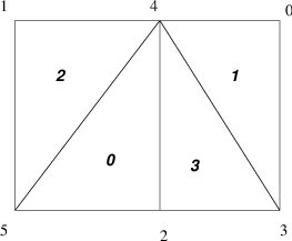
Fig. 6 Numbering on Simple Unstructured Grid#
This, of course, assumes that one has already distributed the grid (graph) information among the processes. The details of this initial distribution is not important; it could be simply determined by assigning to the first process the first \(n_0\) nodes from a file, the second process the next \(n_1\) nodes, etc.
For example, we demonstrate the form of the ia and ja for a
triangular grid where we
partition by element (triangle)
Process 0:
mlocal = 2,n = 4,ja =``{2,3, 3},ia ={0,2,3}Process 1:
mlocal = 2,n = 4,ja =``{0, 0,1},ia =``{0,1,3}
Note that elements are not connected to themselves and we only indicate edge connections (in some contexts single vertex connections between elements may also be included). We use a space above to denote the transition between rows in the matrix; and
partition by vertex.
Process 0:
mlocal = 3,n = 6,ja =``{3,4, 4,5, 3,4,5},ia =``{0, 2, 4, 7}Process 1:
mlocal = 3,n = 6,ja =``{0,2, 4, 0,1,2,3,5, 1,2,4},ia =``{0, 3, 8, 11}.
Once the connectivity matrix has been created the following code will generate the renumbering required for the new partition
MatPartitioningCreate(MPI_Comm comm,MatPartitioning *part);
MatPartitioningSetAdjacency(MatPartitioning part,Mat Adj);
MatPartitioningSetFromOptions(MatPartitioning part);
MatPartitioningApply(MatPartitioning part,IS *is);
MatPartitioningDestroy(MatPartitioning *part);
MatDestroy(Mat *Adj);
ISPartitioningToNumbering(IS is,IS *isg);
The resulting isg contains for each local node the new global number
of that node. The resulting is contains the new process number that
each local node has been assigned to.
Now that a new numbering of the nodes has been determined, one must renumber all the nodes and migrate the grid information to the correct process. The command
AOCreateBasicIS(isg,NULL,&ao);
generates, see Application Orderings, an AO object that can be
used in conjunction with the is and isg to move the relevant
grid information to the correct process and renumber the nodes etc. In
this context, the new ordering is the “application” ordering so
AOPetscToApplication() converts old global indices to new global
indices and AOApplicationToPetsc() converts new global indices back
to old global indices.
PETSc does not currently provide tools that completely manage the migration and node renumbering, since it will be dependent on the particular data structure you use to store the grid information and the type of grid information that you need for your application. We do plan to include more support for this in the future, but designing the appropriate general user interface and providing a scalable implementation that can be used for a wide variety of different grids requires a great deal of time.
See Finite Difference Jacobian Approximations and Matrix Factorization for discussions on performing graph coloring and computing graph reorderings to reduce fill in sparse matrix factorizations.
Jennifer B Erway and Roummel F Marcia. On solving large-scale limited-memory quasi-newton equations. Linear Algebra and its Applications, 515:196–225, 2017.
Jennifer B Erway and Roummel F Marcia. On solving large-scale limited-memory quasi-Newton equations. Linear Algebra and its Applications, 515:196–225, 2017.
J. C. Gilbert and C. Lemarechal. Some numerical experiments with variable-storage quasi-newton algorithms. Mathematical Programming, 45:407–434, 1989.